Laboratory two

Problem One: FIR Design from Ideal Filter

(40 points)

A Finite Impulse Response (FIR) filter is a linear shift invariant filter whose impulse response function is a finite-extent discrete signal. For an FIR filter, the output can be determined from its input by means of the convolution sum, expressed as,

With support over the region, , where .

1. Use the Image Processing Toolbox of MATLAB to design a low-pass filter with a given characteristics (defined by each student group). Provide a plot of, both, impulse response and frequency response of the designed filter using a rectangular window.

2. Repeat part 1 above with three different types of additional windows.

SOLUTION:

1) Use the Image Processing Toolbox of MATLAB to design a low-pass filter with a given characteristics (defined by each student group). Provide a plot of, both, impulse response and frequency response of the designed filter using a rectangular window.

The impulse response h(n) is obtained at the output when the input signal is the impulse signal $\delta = [1,0,0,0,\ldots]$ . The impulse signal is defined by

$\displaystyle \delta(n)\isdef \left\{\begin{array}{ll} 1, & n=0 \\ [5pt] 0, & n\neq 0 \\ \end{array}\right..$

If the th tap is denoted b_k, then it is obvious that the impulse response signal is given by

$\displaystyle h(n)\isdef \left\{\begin{array}{ll} 0, & n<0 \\ [5pt] b_n, & 0\leq n\leq M \\ [5pt] 0, & n> M \\ \end{array} \right. \protect$

In other words, the impulse response simply consists of the tap coefficients, prepended and appended by zeros.

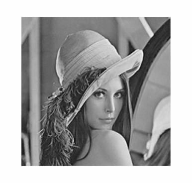
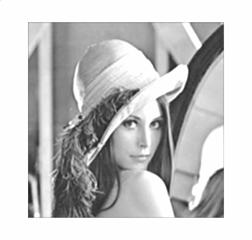
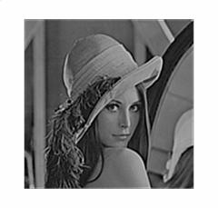
The original image:

1) For the characteristics defined as:

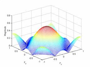
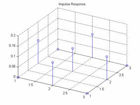
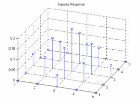
For a frequency space of 3 and a boxcar window of 3 the results are:

Plot of the frequency response and the impulse response:

The output:

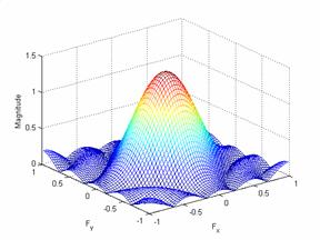
For a frequency space of 5 and a boxcar window of 5 the results are:

Plot of the frequency response and the impulse response:

The output:

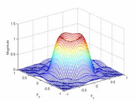
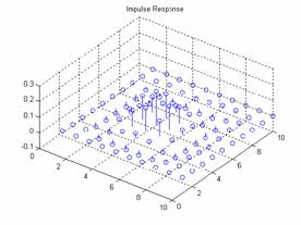
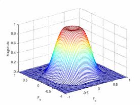
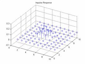
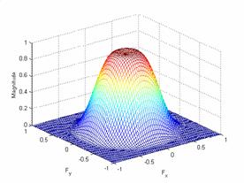
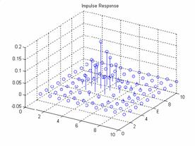
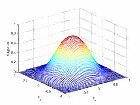
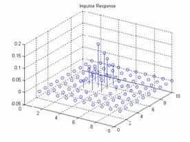
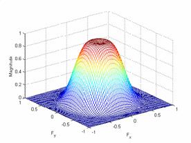
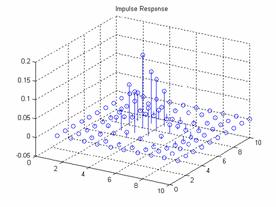
For a frequency space of 10 and a boxcar window of 10 the results are:

Plot of the frequency response and the impulse response:

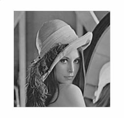
The output:

2) Repeat part 1 above with three different types of additional windows.

Hanning Window:

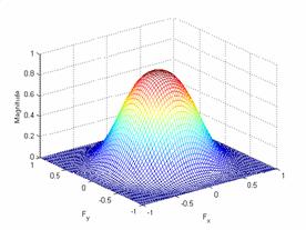
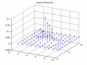
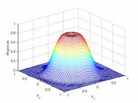
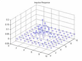
For a frequency space of 10 and a hanning window of 10 the results are:

Plot of the frequency response and the impulse response:

The output:

Hamming Window:

For a frequency space of 10 and a hamming window of 10 the results are:

Plot of the frequency response and the impulse response:

The output:

Blackman Window:

For a frequency space of 10 and a blackman window of 10 the results are:

Plot of the frequency response and the impulse response:

The output:

Blackman-Harris Window:

For a frequency space of 10 and a blackman-harris window of 10 the results are:

Plot of the frequency response and the impulse response:

The output:

Bartlett Window:

For a frequency space of 10 and a bartlett window of 10 the results are:

Plot of the frequency response and the impulse response:

The output:

Gaussian Window:

For a frequency space of 10 and a gaussian window of 10 the results are:

Plot of the frequency response and the impulse response:

The output:

Problem Two: Beamforming techniques

(20 points)

Describe as illustrative as possible the difference between time-domain beamforming and frequency-domain beamforming

SOLUTION:

We will explain one application to sonar where Beamforming is used

The sensor array is composed by the antenna array that detects the signal. Then the signals of the arrays go to the data acquisition that is in charge of digitizing the data. Then the beam forming block generate defined beams from onmielement data (this will be explained better later). The detection processing extract the signal eliminating the noise and the averberation.. Display processing is how the data will be used.

The application is sonar oriented but theory is the same to other applications. Here there is an array of hydrophones receiving signals from an acoustic signal in the far field. The problem here is that the phones across the array receive signals with different time delays, so the phone outputs are not coherent and the summer output drops.

TIME DOMAIN SONAR BEAMFORMING:

In the next figure is shown how the displacement of the source affects the output signal of the array. At the first figure the source is perpendicular to the array plane and for this reason the delay of all the phone is zero, it maximize the output of the whole array. At the second figure the source is moved from the perpendicular and now we can see there are different phase for each signal of the phones. We need to correct this, to do that we could implement a time delay units on each one of the phones, with this units the incoming signal could be adjusted to have a maximum value, simulating the perpendicular conditions.

Conceptually it works but in Sonar applications the delay of the sonar signals is too high and it makes that orientation of the array to the signal is a difficult problem. In order to solve this other strategies must be taken in account. One if manage the delay fo the signals with accelerometer measurement that compensate the time delay. Other strategy is applying oversampling to the data and/or using FIR interpolators.

FREQUENCY DOMAIN SONAR BEAMFORMING:

The main aim of using frequency domain techniques for Sonar Beamforming is to reduce the amount of hardware needed. The time domain Beamforming its efficient with small number of channels array, up to 128 phones and becomes unwieldy for large arrays.

There are several classes of frequency domain Beamforming:

“Conventional” Beamforming where the array element data is essentially time delayed and added to form beams, equivalent to spatial FIR filter.
adaptive beamforming, where more complicated matrix arithmetic is used to suppress interfering signals and to obtain better estimates of wanted targets.
high resolution beamforming, where in a very general sense target signal-to-noise is traded to obtain better array spatial resolution.

NARROW BAND BEAM FORMING:

If the beamformer is required to operate at a single frequency, then the time delay steering system outlined above can be replaced by a phase delay approach. Time delay Beamforming could be written as:

Where:

N: number of hydrophones.

W_k: is the array shading function.

f_k(t): is the time domain k^th data element.

τ_k,_r: is the time delay applied to the k^th element data for the r^th beam.

for the k^th sensor in the array:

Here we must apply an adjustment in the phase of the beamformer in the frequency domain in order to adjust the output of the sensor to the maximum.

CONCLUSION: The main difference between Time domain Beamforming is that in time domain beam forming qe apply a delay in time of the signal and in the Frequency domain Beamforming we apply a product by exp(-jkφ) to compensate the phase difference between the signal of each sensor.
Problem Three: Short-time Fourier transform

(20 points)

Use the cyclic convolution to provide a mathematical formulation of a cyclic version of the filter method of the short-time Fourier transform.

Solution:

Let the sequences be defined as follows:

Let define the following padding operator:

Where:

So let

Let

It’s the Circular Convolution Operation, and using the commutative property of the Circular Convolution we obtain the following:

; where, denotes the circular convolution.

Problem Four: Discrete Fourier Transform

(25 points)

Provide a mathematical description (through demonstration) of four properties of the two-dimensional discrete Fourier transform.

SOLUTION:

TRANSLATION

SEPARABILITY:

Where:

and

PERIODICITY:

LINEARITY:

Given g and h

CIRCULAR TIME SHIFTING:

Problem Two:

(25 points) An ideal low-pass continuous two-dimensional filter has the value of “one” in its pass-band and the value of “zero” after its cut-off frequencies and . Use the time-domain convolution theorem to obtain the output signal, in object domain, of the filter if the input signal is given by the equation below.

Use the following Fourier transform identity:

SOLUTION:

Using the time domain convolution theorem. A convolution in time equals to the inverse Fourier transform of the product of the Fourier Transforms of the input and the impulse response of the filter.

Input Signal Low Pass Filter response

Product of Input and Filter. Output of the System

Then the output of the Filter to the input x(m_x,m_y) is:

Problem Three:

A. (20 points) Write in matrix form the computation of the DFT of the following signal array:

SOLUTION:

On this point we make a variation of the solution, we use the kronecker product and circulant matrix to compute the circular convolution just as a way to try another way to the same result.

The Fourier Matrix for Z₂:

Using Kronecker products:

One-dimensional array scattering operator: (anti-lexicographic)

Applied to the signal array:

Two-dimensional array gathering operator:

DTF:

B. (20 points) Compute the cyclic convolution, using any desired method, of the following two arrays given below. Remember that the cyclic convolution is a commutative, linear operation.